Chapter 5 Linear Discriminant Analysis (LDA)

5.1 TL;DR

What it does: Separates observations into categories, similar logistic regression, but creating actual groups (separated by a line) rather than per-observation probabilities
When to do it: When exploring various classifiers to see which works best for a given data set
How to do it: With the lda() function from the MASS library, using training and testing sets
How to assess it: Assess the accuracy of the predictions on the test set after training

5.2 What it does

Similar to principal component analysys (PCA), LDA reduces dimensionality and finds the best single axis to separate two (or more) groups of observations into categories using a least-squares method of distance from a mean. Like PCA, it returns a set of new axes for the data, organized by importance, so that the first axis is the one that explains the largest amount of variance, and so on, down to \(p - 1\) axes where \(p\) is the number of categories/dimensions.

So, LDA will return 3 axes for a set of observations with 4 categories, or 1 for a set of observations with 2 categories. Each axis will have a loading score that indicates which variables had the biggest impacts on it.

5.3 When to do it

When you want to see if it will work better than other classification methods! It should always be tried along with other classifiers like logistic regression, quadratic discriminant analysis, and Naive Bayes.

5.4 How to do it

Again, using the Boston data from the logistic regression chapter:

data(Boston)
boston <- Boston %>%
  mutate(
    # Create the categorical crim_above_med response variable
    crim_above_med = as.factor(ifelse(crim > median(crim), "Yes", "No")),
  )

We again split the data into training and test sets:

set.seed(1235)
boston.training <- rep(FALSE, nrow(boston))
boston.training[sample(nrow(boston), nrow(boston) * 0.8)] <- TRUE
boston.test <- !boston.training

And fit the above model to the training data using the lda() function from the MASS library¹ (note: there is no family argument as with glm() in logistic regression, but the calls are otherwise identical):

boston_lda.fits <-
  lda(
    crim_above_med ~ nox,
    data = boston,
    subset = boston.training,
  )

5.5 How to assess it

The fit can be directly examined:

boston_lda.fits

## Call:
## lda(crim_above_med ~ nox, data = boston, , subset = boston.training)
## 
## Prior probabilities of groups:
##        No       Yes 
## 0.5247525 0.4752475 
## 
## Group means:
##           nox
## No  0.4710519
## Yes 0.6357865
## 
## Coefficients of linear discriminants:
##          LD1
## nox 12.29052

In the above output, the Prior probabilities of groups information is just the percentage of observations in each of the outcome categories:

> mean(boston[boston.training,]$crim_above_med == "Yes")
[1] 0.4752475
> mean(boston[boston.training,]$crim_above_med == "No")
[1] 0.5247525

The Group means section shows the means of the predictor variable (nox in this case) for each of the categories:

boston[boston.training, ] %>%
  group_by(crim_above_med) %>%
  summarize("Group means" = mean(nox))

## # A tibble: 2 × 2
##   crim_above_med `Group means`
##   <fct>                  <dbl>
## 1 No                     0.471
## 2 Yes                    0.636

And the “Coefficient” is the linear coefficient for the predictor variable nox, which determines the slope of the line that separates the categories.

The fit can be plotted:

plot(boston_lda.fits)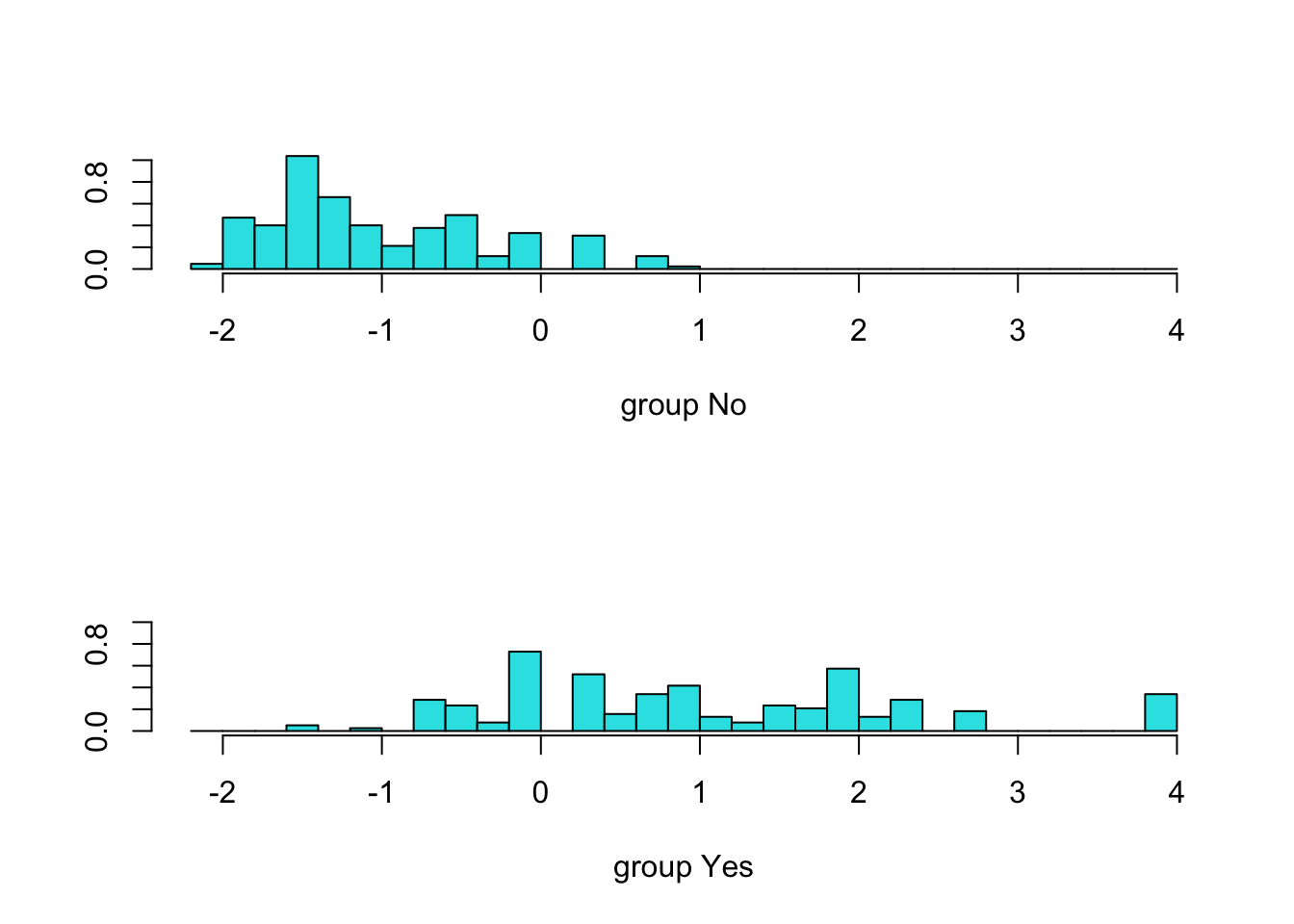

The fit should be used to predict the test data, and the model can be assessed on its results:

boston_lda.pred <- predict(boston_lda.fits, boston[boston.test, ])
table(boston_lda.pred$class, boston[boston.test, ]$crim_above_med)

##      
##       No Yes
##   No  38  12
##   Yes  3  49

In this example, LDA made the correct categorization 87 times out of 102, with 3 false positives and 12 false negatives. Again, we can compute the prediction accuracy by the mean of the correct-to-wrong guesses:

mean(boston_lda.pred$class == boston[boston.test, ]$crim_above_med)

## [1] 0.8529412

If the accuracy rate is good enough for your purposes, you can use the fit in the same manner to make predictions for new data.

5.6 Where to learn more

Chapter 4.4.1 - 4.4.2 in James et al. (2021)
StatQuest: Linear Discriminant Analysis

References

James, Gareth, Daniela Witten, Trevor Hastie, and Robert Tibshirani. 2021. An Introduction to Statistical Learning. 2nd ed. Springer. https://link.springer.com/book/10.1007/978-1-0716-1418-1.

Note to my fellow New Englanders: the MASS library is named for a book titled “Modern Applied Statistics with S”, and although it does contain an earlier version of the Boston dataset (among many others), it has nothing to do with Massachusetts, and our Boston dataset comes from the ISLR2 library.↩︎