Chapter 3 Multiple Linear Regression
3.1 TL;DR
- What it does
- Looks to see how well multiple predictor variables predict an outcome, like how well do years of education and age predict salary?
- When to do it
- When a simple linear regression doesn’t provide a good enough explanation of variance, and you want to see if adding additional variables provides a better one
- How to do it
-
With the
lm()function, utilizing more than one predictor - How to assess it
- Look for significant \(p\)-values for the predictors, and a reasonable adjusted-\(R^2\)
3.2 What it does
Multiple linear regression is the first natural extension of simple linear regression. It allows for more than one predictor variable to be specified. It is also possible to combine predictors in interactions, to find out if combinations of predictors have different effects than simply adding them to the model. XXX explain/demo
3.3 When to do it
Use multiple linear regression when a simple linear regression doesn’t provide a good enough explanation of the variance you’re observing, and you want to see if adding more predictors provides a better fit. Typically, this would be in response to either a low \(R^2\) that leaves a lot of unexplained variance, or even just a visual conclusion drawn from seeing a plot of a linear model with an unsatisfactory regression line.
3.4 How to do it
Use the same lm() function, with more than one predictor in the formula.
lm.fit <- lm(medv ~ lstat + age, data = Boston)
plot(Boston$lstat, Boston$medv)
abline(lm.fit, lwd = 3, col = "red")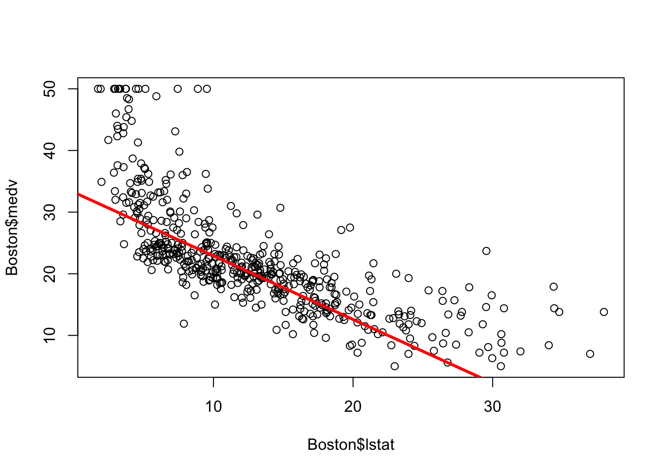
As with simplr linear regression, the results of the regression are stored in the output of lm(), and may be viewed with summary():
summary(lm.fit)##
## Call:
## lm(formula = medv ~ lstat + age, data = Boston)
##
## Residuals:
## Min 1Q Median 3Q Max
## -15.981 -3.978 -1.283 1.968 23.158
##
## Coefficients:
## Estimate Std. Error t value Pr(>|t|)
## (Intercept) 33.22276 0.73085 45.458 < 2e-16 ***
## lstat -1.03207 0.04819 -21.416 < 2e-16 ***
## age 0.03454 0.01223 2.826 0.00491 **
## ---
## Signif. codes: 0 '***' 0.001 '**' 0.01 '*' 0.05 '.' 0.1 ' ' 1
##
## Residual standard error: 6.173 on 503 degrees of freedom
## Multiple R-squared: 0.5513, Adjusted R-squared: 0.5495
## F-statistic: 309 on 2 and 503 DF, p-value: < 2.2e-16All of the same parameters are there, with the addition of one coefficient line for each parameter specified in the model. Each coefficient has its own estimate, standard error, \(t\) value and \(p\) value, and should be evaluated independently.
The main task is to get the ideal subset of parameters that provide the best fit, which can involve a lot of trial and error. Forward selection involves starting with a null model (no parameters) and trying all available parameters to see which has the lowest p-value, and adding that and continuing until the parameters are no longer significant or don’t reduce the adjusted \(R^2\); Backward selection starts with all parameters and removes the least significant one at a time until all remaining parameters are significant; Mixed selection starts with forward selection but also removes parameters that lose their significance along the way.
Other tidbits:
- interaction terms can be specified with syntax like
lstat * age, which addslstat,ageandlstat * ageas predictors; if an interaction is significant but an individual predictor from the interaction isn’t, it should still be left in the model - nonlinear transformations like \(\text{age}^2\) can be added by escaping them inside the
I()function, likeI(age^2), to escape the^character inside the formula
3.5 How to assess it
With the exception of the additional information for each parameter, the assessment is the same as for simple linear regression.
In the example above, we see that the addition of age only added a tiny bit of improvement to the model from the simple linear regression on just lstat. Other variables, or combinations of variables, might do a better job.
3.6 Where to learn more
- Chapter 3.2 in James et al. (2021)