Chapter 6 Quadratic Discriminant Analysis
6.1 TL;DR
- What it does
- Assigns observations to categories like linear discriminant analysis, but with a more flexible / curved boundary rather than a straight line
- When to do it
- When linear discriminant analysis isn’t giving good enough results (esp. if the dataset is very large)
- How to do it
-
With the
qda()function from the MASS library, using training and testing sets - How to assess it
- Assess the accuracy of the predictions on the test set after training
6.2 What it does
Just like linear discriminant analysis, quadratic discriminant analysis attempts to separate observations into two or more classes or categories, but it allows for a curved boundary between the classes. Which approach gives better results depends on the shape of the Bayes decision boundary for any particular dataset. The following figure from James et al. (2021) shows the two approaches:
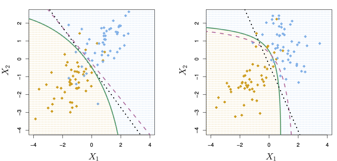
Figure 6.1: LDA and QDA plots (source: James et al. (2021), p. 154)
The purple dashed line in both diagrams shows the Bayes decision boundary. The LDA line in the left plot shows this class separation line as straight; the QDA line on the right is curved.
6.3 When to do it
Use QDA when the linear separation of linear discriminant analysis isn’t giving good enough results, and you think a curved (or quadratic) line might fit better.
6.4 How to do it
Exactly like linear discriminant analysis, except for the qda() call instead of lda(). Train the model on training data, assess it against test data.
data(Boston)
boston <- Boston %>%
  mutate(
    # Create the categorical crim_above_med response variable
    crim_above_med = as.factor(ifelse(crim > median(crim), "Yes", "No")),
  )
We again split the data into training and test sets:
set.seed(1235)
boston.training <- rep(FALSE, nrow(boston))
boston.training[sample(nrow(boston), nrow(boston) * 0.8)] <- TRUE
boston.test <- !boston.training
and call qda() on the training data:
boston_qda.fits <-
  qda(
    crim_above_med ~ nox,
    data = boston,
    subset = boston.training,
  )
6.5 How to assess it
As with lda(), the resulting fit can be directly examined:
boston_qda.fits## Call:
## qda(crim_above_med ~ nox, data = boston, , subset = boston.training)
##
## Prior probabilities of groups:
## No Yes
## 0.5247525 0.4752475
##
## Group means:
## nox
## No 0.4710519
## Yes 0.6357865Note that in this example, the Prior probabilities of groups and Group means assessments are identical to those from lda(). There is no linear discriminant coefficient, because this is not a linear discriminant! The rest of the output is identical.
We then call predict on the QDA fit, to predict the crim_above_med variable from nox:
boston_qda.pred <- predict(boston_qda.fits, boston[boston.test, ])
table(boston_qda.pred$class, boston[boston.test, ]$crim_above_med)
##
## No Yes
## No 38 12
## Yes 3 49In this example, just like LDA, QDA made the correct categorization 87 times out of 102, with 3 false positives and 12 false negatives. And again, we can compute the prediction accuracy by the mean of the correct-to-wrong guesses:
mean(boston_qda.pred$class == boston[boston.test, ]$crim_above_med)## [1] 0.8529412In this case, QDA offered no increase in prediction accuracy over LDA, so there is no reason to prefer it (although it also performed no poorer).
6.6 Where to learn more
- Chapter 4.4.3 in James et al. (2021)