Chapter 4 Logistic Regression

4.1 TL;DR

What it does

Models the probability that an observation falls into one of two categories

When to do it

When you are trying to predict a categorical variable with two possible outcomes, like true/false, instead of something continuous like in linear regression

How to do it

With the glm() function, specifying family = "binomial"

How to assess it

Look for a significant \(p\)-value for the predictor, and assess its accuracy against training data

4.2 What it does

Logistic regression is used to make a prediction about whether an observation falls into one of two categories. This is an alternative to linear regression, which predicts a continuous outcome. A logistic regression results in a model that gives the probability of Y given X.

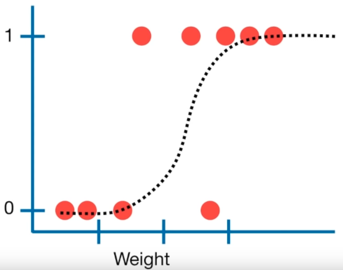
Figure 4.1: Linear regression plot (source: StatQuest)

4.3 When to do it

As the TL;DR says: When you are trying to predict a categorical variable with two possible outcomes, like true/false, instead of something continuous.

4.4 How to do it

First, it’s important to note that logistic regression will give better results when the model is fit using held out or training data, and then tested against other data, to help avoid overfitting. It is not required, but it’s recommended where possible.

First, before that, fit a model using glm(), making sure in this case that we have a categorical value to test for:

data(Boston)
boston <- Boston %>%
  mutate(
    # Create the categorical crim_above_med response variable
    crim_above_med = as.factor(ifelse(crim > median(crim), "Yes", "No")),
    # Also make a numeric version of crim_above_med for the plot
    crim_above_med_num = ifelse(crim > median(crim), 1, 0)
  )
boston.fits <- glm(crim_above_med ~ nox, data = boston, family = binomial)
summary(boston.fits)

## 
## Call:
## glm(formula = crim_above_med ~ nox, family = binomial, data = boston)
## 
## Deviance Residuals: 
##      Min        1Q    Median        3Q       Max  
## -2.27324  -0.37245  -0.06847   0.39620   2.53124  
## 
## Coefficients:
##             Estimate Std. Error z value Pr(>|z|)    
## (Intercept)  -15.818      1.386  -11.41   <2e-16 ***
## nox           29.365      2.599   11.30   <2e-16 ***
## ---
## Signif. codes:  0 '***' 0.001 '**' 0.01 '*' 0.05 '.' 0.1 ' ' 1
## 
## (Dispersion parameter for binomial family taken to be 1)
## 
##     Null deviance: 701.46  on 505  degrees of freedom
## Residual deviance: 320.39  on 504  degrees of freedom
## AIC: 324.39
## 
## Number of Fisher Scoring iterations: 6

We can see the that \(p\) value for the nox variable is nearly 0, suggesting a strong association between nox and crim_above_med.

Now split the data into training and test sets, using, say, 80% of the data for training:

set.seed(1235)
boston.training <- rep(FALSE, nrow(boston))
boston.training[sample(nrow(boston), nrow(boston) * 0.8)] <- TRUE
boston.test <- !boston.training

Fit the above model to the training data:

boston.fits <-
  glm(
    crim_above_med ~ nox,
    data = boston,
    subset = boston.training,
    family = binomial
  )

And use the fit to predict the test data with predict():

boston.probs <- predict(boston.fits, boston[boston.test,], type = "response")

4.5 How to assess it

Assess the accuracy of the predictions by building a confusion matrix, using the same values (“No” and “Yes” in this case) as contained in the outcome variable we want to predict:

boston.pred <- rep("No", sum(boston.test))
boston.pred[boston.probs > 0.5] <- "Yes"
table(boston.pred, boston[boston.test,]$crim_above_med)

##            
## boston.pred No Yes
##         No  36  12
##         Yes  5  49

The above table shows that the model correctly predicted crim_above_med from nox 85 times out of 102, with 5 false positives and 12 false negatives. The accuracy of the model can be computed via the mean() of how often the predictions match the test data, a neat trick:

mean(boston.pred == boston[boston.test,]$crim_above_med)

## [1] 0.8333333

The regression can be plotted with ggplot2 and the stat_smooth() function, utilizing the glm method, like so:

ggplot(boston, aes(x = nox, y = crim_above_med_num)) +
  geom_point(alpha = .5) +
  stat_smooth(
    method = "glm",
    formula = y ~ x,
    se = FALSE,
    method.args = list(family = binomial),
    col = "red",
    lty = 2
  )

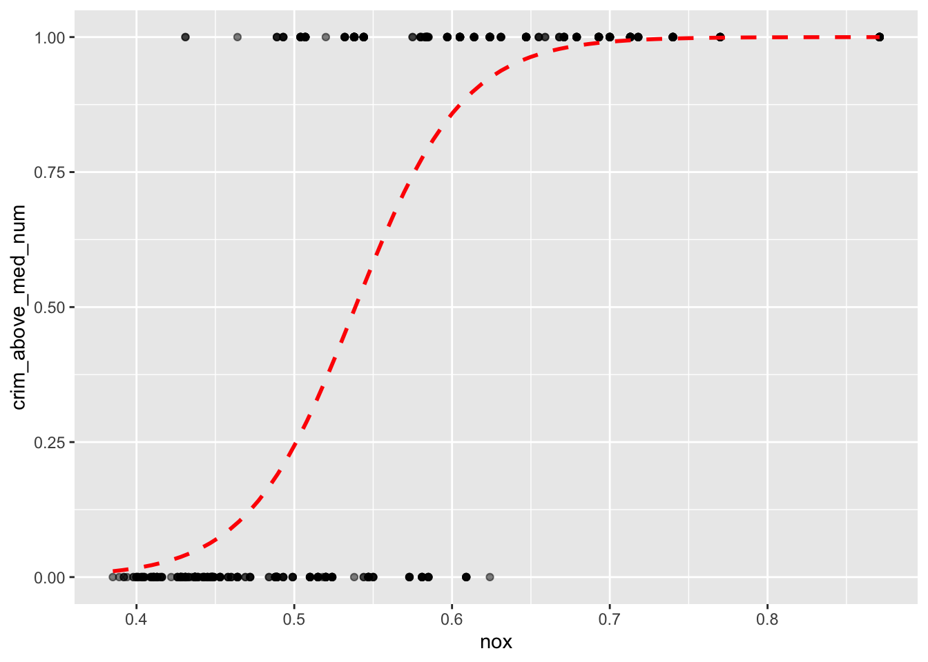
This shows that an observation with a nox value of 0.6 would have around a 90% probability of crim_above_med being true, or 1, while an observation with a nox value of 0.5 would only have around a 25% probability of crim_above_med being true.

4.6 Where to learn more

• Chapter 4 - 4.4 in James et al. (2021)
• StatQuest: Logistic Regression

4.7 Notes

Like with linear regression, the “multiple” flavor of logistic regression works much the same way, with the specification of additional predictors in the formula, and so doesn’t really warrant a whole chapter of its own. The selection of variables requires some effort, and is addressed under best subser selection.

References

James, Gareth, Daniela Witten, Trevor Hastie, and Robert Tibshirani. 2021. An Introduction to Statistical Learning. 2nd ed. Springer. https://link.springer.com/book/10.1007/978-1-0716-1418-1.